Confidence band

The present implementation of randomization inference is designed for fast computation of both confidence bounds and bands for the coefficient. In fact, computing bounds is the default setting.¹ To illustrate this feature, I follow the example provided in the documentation for the Stata implementation.

Tip

Code available in the repository.

Data

I use a toy dataset with 100 observations. Treatment is deterministically assigned so that half the observations are treated, and the outcome is generated as a linear function of treatment with a true treatment effect of 0.3 plus standard normal noise. The data are then used to estimate a simple OLS regression of the outcome on treatment and exported to CSV for use in CI-band examples.

Stata

The code is directly taken from Stata’s ritest github repository. I made a few edits to make it easier to compare, but it remains computationally equivalent to the example presented in the repository.

Run ritest to find which hypotheses for the treatment effect in [-1,1] can[not] be rejected.

tempfile gridsearch

postfile pf TE pval using `gridsearch'

forval i=-1(0.05)1 {

    qui ritest treatment (_b[treatment]), reps(500) null(y `i') seed(123): reg y treatment // tc: run with _b[treatment] only to compare


    mat pval = r(p)
    post pf (`i') (pval[1,1])
}
postclose pf

Plot the bands, with ugly vertical lines at \(-0.2\), \(0.2\), and \(0.6\) to help comparison with the Python results:

use `gridsearch', clear

tw line pval TE , yline(0.05) xline(-0.2 0.2 0.6)

For additional context, for a null of equality to zero,

ritest treatment (_b[treatment]), nodots reps(500) seed(123): ///
           reg y treatment

this is the randomization inference result:

      Command: regress y treatment
        _pm_1: _b[treatment]
  res. var(s):  treatment
   Resampling:  Permuting treatment
Clust. var(s):  __000001
     Clusters:  100
Strata var(s):  none
       Strata:  1

------------------------------------------------------------------------------
T            |     T(obs)       c       n   p=c/n   SE(p) [95% Conf. Interval]
-------------+----------------------------------------------------------------
       _pm_1 |   .2019068     181     500  0.3620  0.0215  .3198005    .405842
------------------------------------------------------------------------------
Note: Confidence interval is with respect to p=c/n.
Note: c = #{|T| >= |T(obs)|}

The confidence bands, which are obtained by running ritest with a set of different non-zero nulls, are shown below:

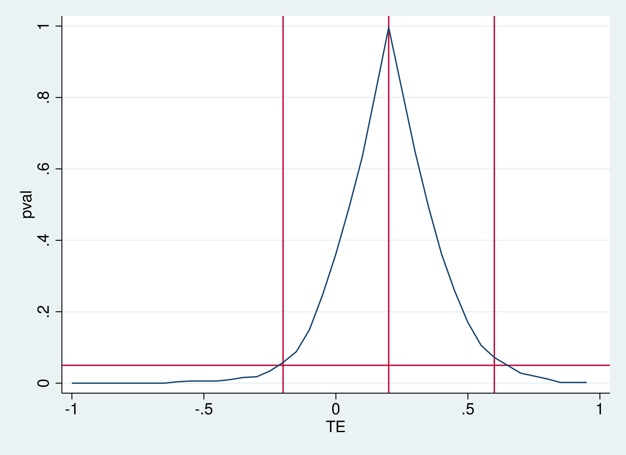
where the y-axis represents randomization inference \(p\)-values, and the x-axis represent treatment effects. The blue line maps different treatment effects to \(p\)-values. The horizontal line is drawn at 0.05, corresponding to the most common significance level. These plot shows that the point estimate is about \(0.2\) and the confidence interval is roughly \([-0.2,0.6]\).

138 seconds, which is about 2.3 minutes.

Python

Run ritest, set ci_mode="grid" to get confidence bands:

    res = ritest(
        df=df,
        permute_var="treatment",
        formula="y ~ treatment",
        stat="treatment",
        reps=500,
        ci_mode="band",
        seed=123,
    )

For additional context, this is the result of the randomization inference for a null of equality to zero:

Randomization Inference Result
===============================

Coefficient
-----------
Observed effect (β̂):   0.2019
Coefficient CI bounds: [-0.1886, 0.5873]
Coefficient CI band:   available (fast-linear)

Permutation test
----------------
Tail (alternative):     two-sided
p-value:                0.3100 (31.0%)
P-value CI @ α=0.050: [0.2697, 0.3526]
As-or-more extreme:     155 / 500

Test configuration
------------------
Strata:                 —
Clusters:               —
Weights:                no

Settings
--------
alpha:                  0.050
seed:                   123
ci_method:              clopper-pearson
ci_mode:                band
n_jobs:                 4

The corresponding confidence band is shown below:

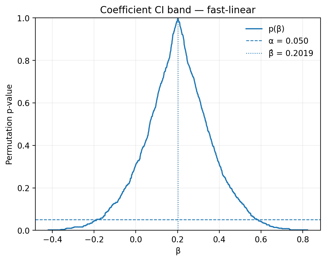
0.06 seconds.

Footnotes

Implementations of randomization inference typically report a \(p\)-value and a confidence interval (or bounds) for that \(p\)-value. This is at odds with the confidence interval you would normally get from a regression, which is a confidence interval for the coefficient.↩︎